Table of Contents
- Introduction
- Monte Carlo Simulation Basics
- Using Random Sampling to Estimate Pi
- A Python Implementation
- Conclusion
- References and Further Reading
- Monte Carlo Interview Questions
Introduction
How can we estimate the value of $\pi$? While we know $\pi$ is irrational and cannot be expressed as a finite closed formula, approximations like $3.14$ or $22/7$ are widely used. But what if we want a systematic, simulation-based method to approximate $\pi$ with arbitrary precision?
Monte Carlo methods provide exactly this. By exploiting randomness and statistical principles, we can approximate $\pi$ in a surprisingly elegant way. This tutorial walks step by step through the mathematics and Python code.
Monte Carlo Simulation Basics
Monte Carlo methods rely on random sampling and the central limit theorem (CLT) to estimate expectations. Indeed the CLT states that for $(X_i)_{i=1}^n$ $n$ independent and identically distributed random variables :
\[\frac{1}{\sqrt{n}}\sum_{i=1}^{n}(X_i - \mu) \xrightarrow[]{d} N(0, \sigma^2)\]If we can find a random variable $X$ such that $\mathbb{E}[X] = \pi$, then simulating $X$ repeatedly and averaging would us an estimate of $\pi$ ! The more samples we take, the closer we get to the true value, with the rate of convergence governed by the variance of $X$.
But this here is a quant blog. Suppose we want the absolute error to be less than $\varepsilon > 0$ with probability at least $1 - \alpha$. Can we solve this problem ? Answer is yes, but with some maths.

Let’s consider $\text{Var}(X) = \sigma^2$, then by the Central Limit Theorem, the sample mean
\[\hat{\pi}_n = \frac{1}{n} \sum_{i=1}^n X_i\]satisfies
\[\sqrt{n}\,(\hat{\pi}_n - \pi) \xrightarrow[]{d} N(0, \sigma^2).\]This means that for large $n$, the estimation error is approximately normal with variance $\frac{\sigma^2}{n}$. Hence, the standard error of our estimator is
\[\text{SE}(\hat{\pi}_n) = \frac{\sigma}{\sqrt{n}}.\]Using the normal approximation, we require
\[\mathbb{P}\big( |\hat{\pi}_n - \pi| < \varepsilon \big) \approx 1 - \alpha.\]This leads to the condition
\[\frac{\sigma}{\sqrt{n}} z_{1-\alpha/2} \leq \varepsilon,\]where $z_{1-\alpha/2}$ is the $(1 - \alpha/2)$ quantile of the standard normal distribution (for example, $z_{0.975} \approx 1.96$ for a $95\%$ confidence level).
Rearranging gives the required number of runs:
\[n \geq \left( \frac{z_{1-\alpha/2} \cdot \sigma}{\varepsilon} \right)^2.\]This formula provides a practical guideline: once we know or estimate the variance $\sigma^2$ of the Monte Carlo variable, we can determine how many simulations are needed to achieve a desired accuracy $\varepsilon$ with a given confidence level $1 - \alpha$.
Using Random Sampling to Estimate $\pi$
In practice, random number generation typically begins with pseudo-random draws from a uniform distribution, which can be transformed into other distributions. In Python, numpy provides a straightforward way to simulate such values.
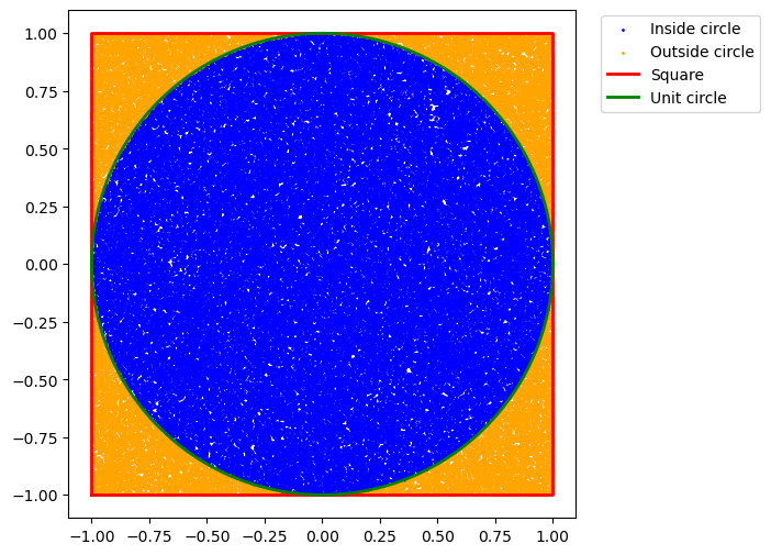
Here is the key idea: let $X_1$ and $X_2$ be two i.i.d. uniform random variables on $[-1, 1]$. The probability that the point $(X_1, X_2)$ falls inside the unit circle is proportional to the ratio between the area of the circle and the area of the square:
\[\mathbb{P}(X_1^2 + X_2^2 \leq 1) = \frac{\text{Area of Circle}}{\text{Area of Square}} = \frac{\pi r^2}{(2r)^2} = \frac{\pi}{4}.\]Thus, if we simulate many points uniformly in the square $[-1, 1]^2$ and check the fraction that lies within the unit circle, multiplying this fraction by 4 yields an approximation of $\pi$.
We can for sure also ask ourself : what is the value of $\sigma_X$?
By definition,
\(\sigma_X = \sqrt{\mathbb{E}[X^2] - \mathbb{E}[X]^2}\)
Here, $X$ is the indicator function of the event ${(X_1, X_2) \in \text{Unit Circle}}$. Since $X$ is an indicator, we have $X^2 = X$, thus :
\[\mathbb{E}[X^2] = \mathbb{E}[X] = \frac{\pi}{4}\]And so we find :
\[\sigma_X = \sqrt{\frac{\pi}{4} - \left(\frac{\pi}{4}\right)^2} = \sqrt{\frac{\pi}{4} \cdot \frac{4 - \pi}{4}} = \sqrt{\frac{\pi (4 - \pi)}{16}}.\]Thus,
\[\sigma_X < \frac{1}{2}.\]A Python Implementation
The implementation is straightforward:
import numpy as np

n = int(1e6)  # number of simulations
x1 = np.random.uniform(-1, 1, n)
x2 = np.random.uniform(-1, 1, n)

# Check which points fall inside the unit circle
inside_circle = x1**2 + x2**2 <= 1

# Estimate of pi
pi_estimate = 4 * inside_circle.mean()
print(pi_estimate)
Running this code with one million points gives a fairly good approximation of $\pi$. Increasing n will further improve accuracy.
Conclusion
Estimating $\pi$ with Monte Carlo is a beautiful demonstration of how probability and geometry intersect. It shows that if we can identify a random variable with an expectation equal to the quantity of interest, then repeated sampling gives us a practical way to approximate it.
References and Further Reading
- Monte Carlo Method — Wikipedia
- Central Limit Theorem — Wikipedia
- Gentle, J. E. (2003). Random Number Generation and Monte Carlo Methods. Springer.
Monte Carlo Interview Questions
1. What is a Monte Carlo simulation, and why is it useful in quantitative finance?
Monte Carlo simulation uses random sampling to approximate complex probabilistic outcomes. In finance, it's used for option pricing, risk management, portfolio optimization, and evaluating scenarios where closed-form solutions are difficult.
2. How does Monte Carlo simulation leverage randomness to approximate deterministic quantities like π?
By generating many random points in a known geometric space (e.g., a square), we can estimate the probability of events (e.g., falling inside a circle). Multiplying this probability by the appropriate factor gives an approximation of π.
3. What role does the Central Limit Theorem play in Monte Carlo methods?
The Central Limit Theorem justifies that the sample mean of independent simulations approximates a normal distribution for large samples, allowing us to compute confidence intervals and error bounds for estimates.
4. How do you determine the number of Monte Carlo simulations needed to achieve a desired accuracy?
Using the standard error formula: \( SE = \sigma / \sqrt{n} \), and desired error \(\varepsilon\) at confidence level \(1-\alpha\), the required simulations are \( n \ge (z_{1-\alpha/2} \cdot \sigma / \varepsilon)^2 \).
5. How can π be estimated using random sampling in a unit square?
Generate uniform random points in $[-1,1]^2$. Count the fraction inside the unit circle. Multiply this fraction by 4 to estimate π: $$ \pi \approx 4 \times frac{\text{points inside circle}}{\text{total points}} $$
6. What is the variance of the Monte Carlo estimator when estimating π?
Using the indicator variable for a point inside the circle: \( \sigma^2 = \frac{\pi}{4}\left(1 - \frac{\pi}{4}\right) \). The standard error of the mean decreases with \(1/\sqrt{n}\).
7. How would you implement a Monte Carlo simulation to estimate π in Python efficiently?
Use vectorized operations in NumPy to generate random points and compute the fraction inside the unit circle. Example:
import numpy as np
n = 1_000_000
x, y = np.random.uniform(-1, 1, n), np.random.uniform(-1, 1, n)
pi_estimate = 4 * ((x**2 + y**2) <= 1).mean()
print(pi_estimate)
8. How can variance reduction techniques improve Monte Carlo estimation?
Techniques like antithetic variates, control variates, and quasi-random sequences reduce estimator variance, improving accuracy without increasing the number of simulations—a critical tool in hedge fund risk modeling.
9. Why is understanding the standard error important in quantitative simulations?
The standard error quantifies the expected fluctuation of the estimate around the true value, allowing quants to construct confidence intervals and assess the reliability of Monte Carlo results.
10. Where are Monte Carlo methods commonly applied in quantitative finance?
Applications include derivative pricing (e.g., options), Value-at-Risk (VaR) calculation, stress testing portfolios, scenario analysis, and simulating complex stochastic processes like interest rates or asset paths.